Reciprocal Function
Transformations
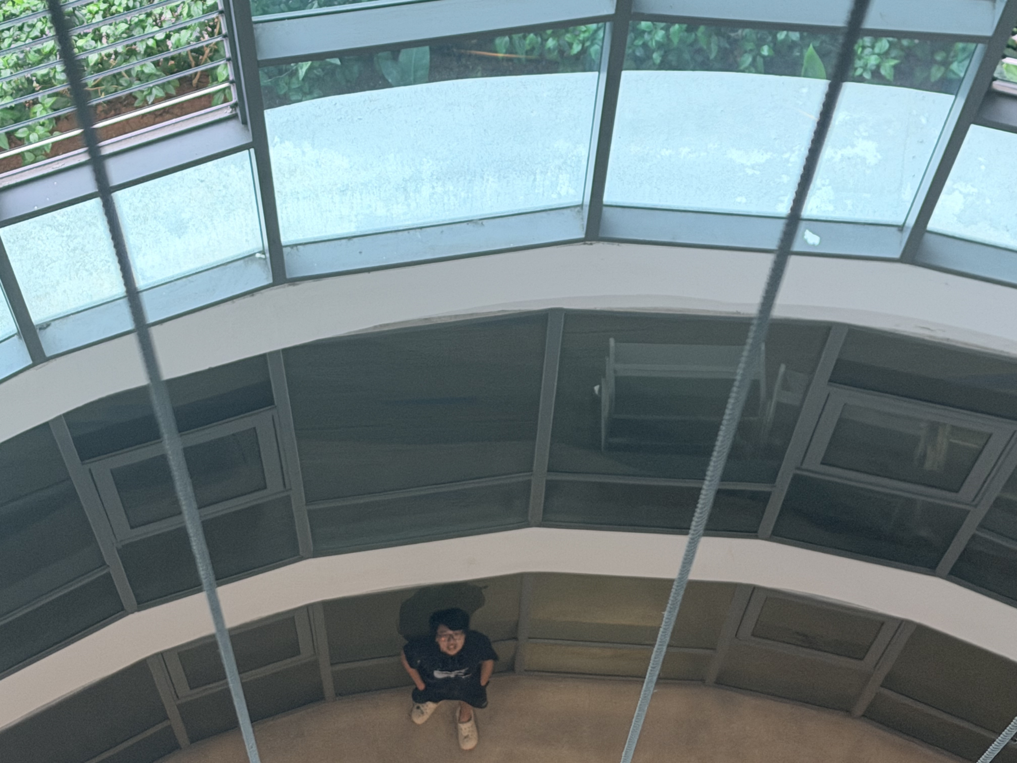
The reason why I picked this photo is that there is a unique feature in the building of the University I study at – a curved ceiling of the passage between two lecture rooms. To start modeling the ceiling's shape using the graph, I noticed that its shape resembled a reciprocal function and decided that the parent graph I will be dealing with should be \( y = \frac{1}{x} \).
Analyzing the graph of this particular function, I saw that its part in my picture was decreasing instead of being increasing, so the part I will deal with will be the right-hand one (when \( x > 0 \)). At the very beginning of the problem solving process I had a great difficulty determining what the exact coefficient of vertical stretching or compression should be due to the fact that the graph was shifted far away from the origin. So what I did first of all is make an adjustment that will make me able to work only with the shape of the graph – I placed the curve in the first quadrant without doing any translations. Having compared the rate of change, I concluded that a vertical stretch, not compression, will be required.
After the shape was determined, I placed the graph back into its original location using translations. I performed a horizontal translation to match the beginning of the graph with where it was located on the graph, followed by a vertical translation that allowed the graph to pass through certain points. The equation I came up with is:
Domain and Range
The domain of the function that I created is:
This is because I constrained the domain to the part of the ceiling which could be seen in the photograph. Reflecting on the whole process, I would have ensured that the entire length of the corridor is seen in the photograph since this would have allowed me to construct a model of the entire curve, not just the one seen in the photograph.
The parent function \( y = \frac{1}{x} \) has a domain of \( D: \{x \in \mathbb{R} \mid x \neq 0\} \) and a range of \( R: \{y \in \mathbb{R} \mid y \neq 0\} \). In other words, this function can be applied to any value except zero and can generate any number but zero. Moreover, there is a vertical asymptote of \( x = 0 \) and a horizontal one of \( y = 0 \), which are not included in the function’s domain because it is undefined at these values. With the help of transformations, I have also obtained asymptotes of \( x = 3 \) (vertical) and \( y = 1 \) (horizontal), yet the restriction of the domain does not allow undefined values in this particular case.
Because of the continuity of the function within the limited domain, the range can be found by finding the value of the function at the ends of the domain. After evaluating at \( x = 3.2 \) and \( x = 5.0 \), the approximate output values are 11 and 2, respectively.
Hence, the range of the function is approximately:
Exponential Function
Transformations
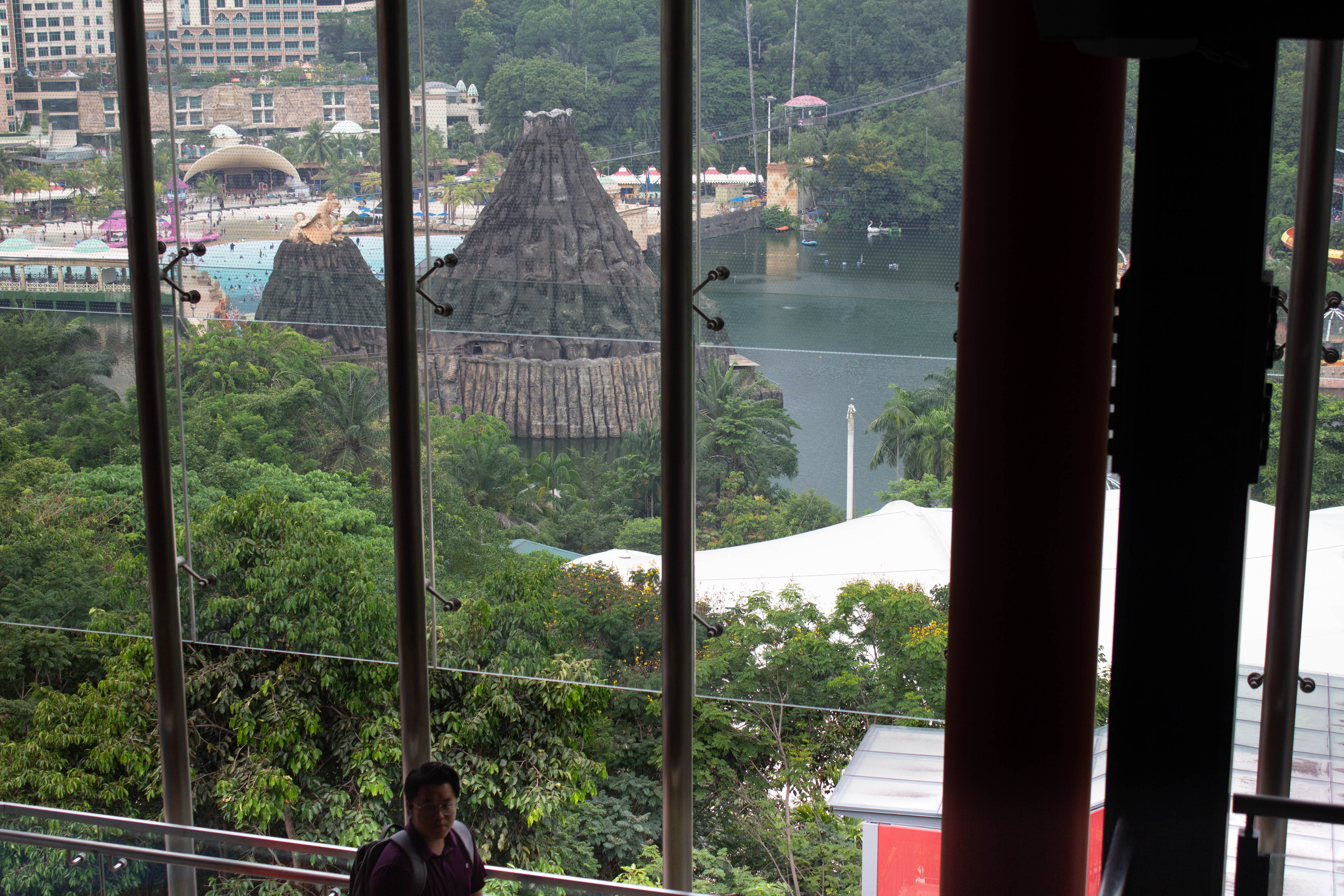
This picture was chosen because I like to hike and take in nature. The outline of the volcano in this picture represents an exponential decay graph very well. In order to create a slope for this volcano, first I needed to figure out that it was similar to an exponential graph; hence, the use of the parent graph \( y = 2^x \).
After looking at the orientation of the graph within the picture, I realized that it was decreasing instead of increasing, meaning there must have been a flip along the y-axis. In this case, I decided to modify the equation to be \( y = 2^{-x} \) to match the orientation of the graph. At first, it was quite hard for me to find the exact horizontal stretch or compression needed because the graph within the picture was situated quite far away from the origin. This made it quite complicated for me to assess how steep it really was. To overcome this problem, I decided to move the graph temporarily within the picture so that the horizontal asymptote would be at \( y = 0 \). This way, I would be able to disregard any translational aspects of the graph and concentrate solely on its shape.
Now that the shape had been set, I translated the graph back into its original position. Firstly, I did this by translating the graph horizontally so that the beginning was at the right point on the graph and then a vertical translation was done, ensuring that the graph passes through certain points. The graph was then modeled by:
Domain and Range
The domain of the function that I created is:
I restricted the domain to the visible part of the volcano's slope. If I were to redo this experiment, I would take an image of the whole volcano so that I could analyze it as one curve. Otherwise, it is not possible to determine how accurate my results will be, since they apply only to the visible part of the volcano.
However, the domain and the range of the parent function are defined as:\( D: \{x \in \mathbb{R}\} \)
\( R: \{y \in \mathbb{R} \mid y > 0\} \)
This is because this function is able to accept all real number values and return any positive real number. It has a horizontal asymptote of \( y = 0 \) where the function approaches zero but cannot equal it. My function also has a horizontal asymptote of \( y = -1 \), but I have limited the domain of the graph to an interval that lies entirely above the asymptote. Thus, the domain of my function is not bounded by an asymptote; hence, I do not need to include one when defining its domain and range.
Because the function is a continuous function over the limited domain, the range of the function would be obtained from evaluating the function at both ends of the domain. The evaluations led me to conclude that my approximate outputs were 0 and -0.5. Therefore, the range of my function is approximately:
Polynomial Function
Transformations
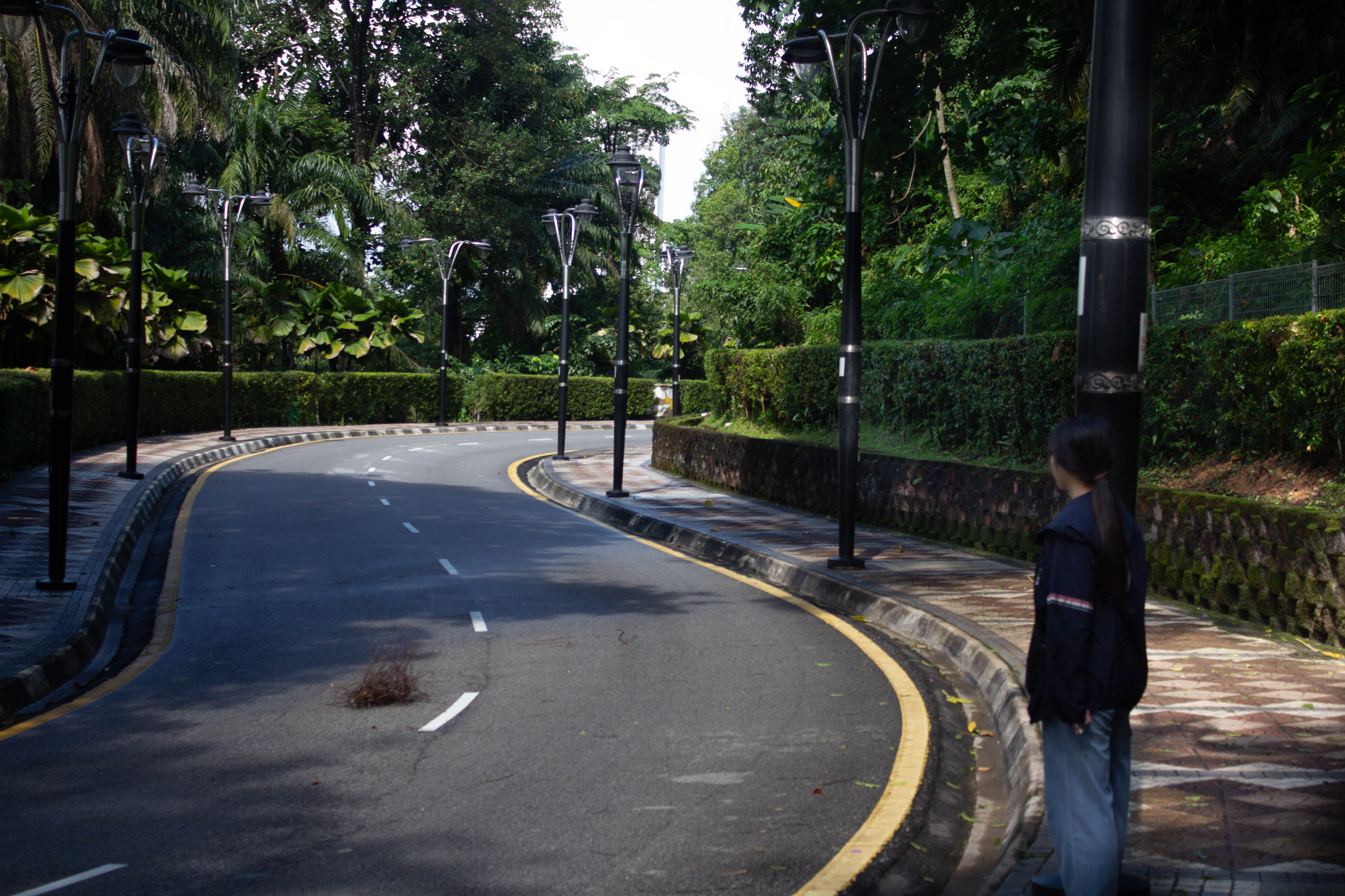
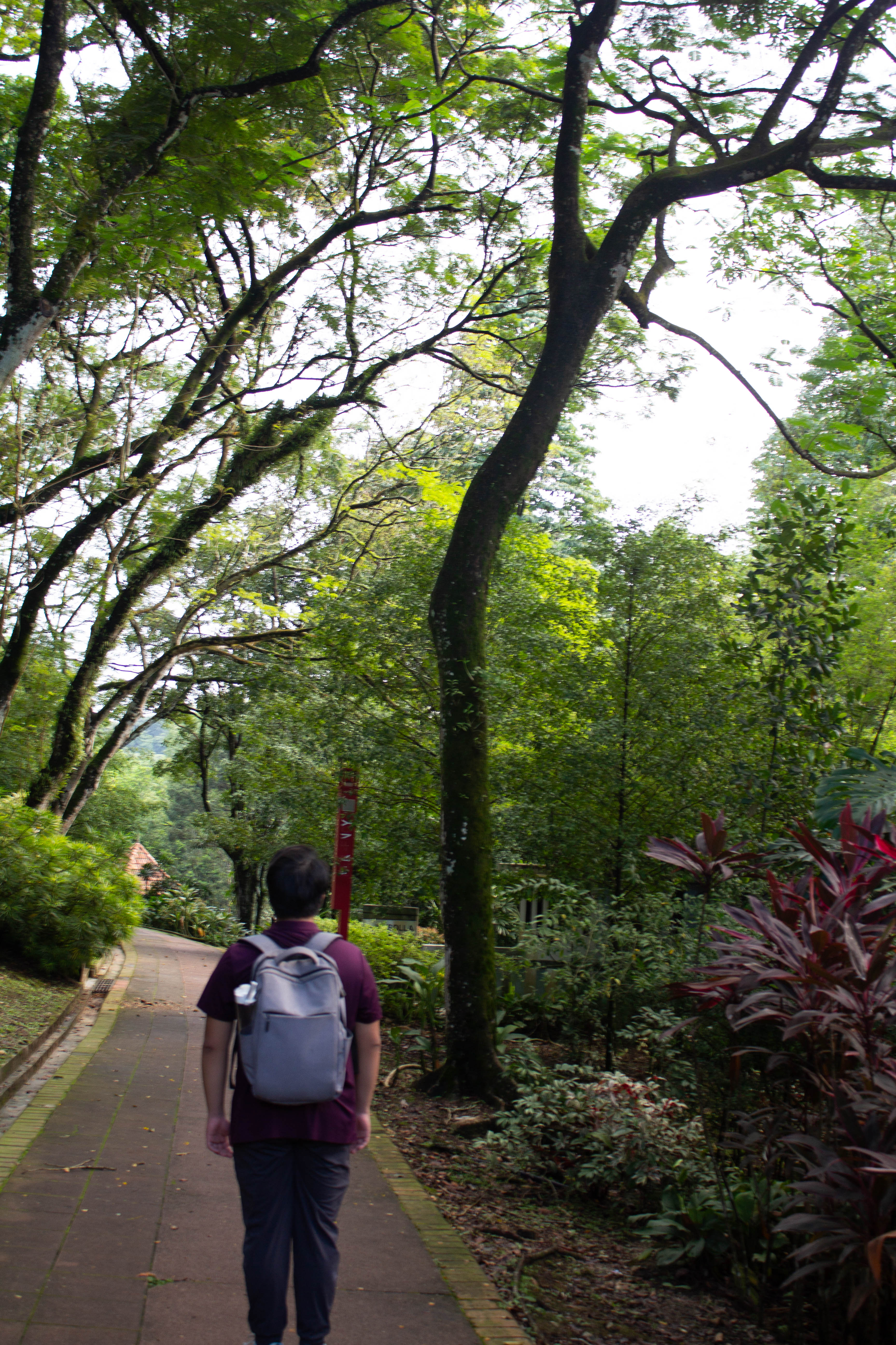
I picked this picture because I go for a walk along this curvy road every weekend, and the smooth nature of its curves reminded me of a quartic polynomial. To find the equation of the road, I realized that the form of the road followed that of a fourth-degree polynomial function, and thus, I decided to start with the parent function \( y = x^4 \).
From analyzing the position of the curve in the picture, I saw that the curve was concave down and not up. From this, I concluded that there must have been a reflection along the x-axis, and thus, I decided to modify my parent function to become \( y = -x^4 \). It took me some time to figure out whether there was a horizontal compression or stretch, considering that the curve in the picture was so far from the origin that it became hard for me to tell the difference. To overcome this problem, I first had to translate the curve so that the vertex coincided with the point \( (0,0) \). Now, all I needed to do was to analyze the shape of the graph, without having to worry about the translation.
Once I had created the shape, I used transformations to put the graph back into its original position. I moved the graph left or right until the vertex aligned itself where it should be according to the photo, and then translated it vertically to pass through specific points. This function modeled the shape of the road in the photograph:
Domain and Range
The domain of the function that I created is:
I restricted the domain to those parts of the road that were seen in the picture. Upon reflection, I think I should have taken a picture where all of the road is seen, enabling me to create a model of the whole thing and not just the part that was seen in the picture.
The parent function \( y = x^4 \) has a domain of \( D: \{x \in \mathbb{R}\} \) and a range of \( R: \{y \in \mathbb{R} \mid y \ge 0\} \). This indicates that the function is defined for all real numbers and can have all real outputs starting from zero. The parent function also has a vertex at point \( (0,0) \) where it attains its lowest value. In the case of my function, the vertex lies at point \( (4,3) \).
As the function is continuous within the restricted domain, its range can be calculated by substituting values of \( x \) at both ends of the domain and at the vertex. Substituting \( x \) as \( 2 \), \( 4 \), and \( 6 \) gave me approximations of the output values as \( 1 \), \( 3 \), and \( 1 \) respectively.
Therefore, the range of my function is approximately:
Tangent Function
Transformations
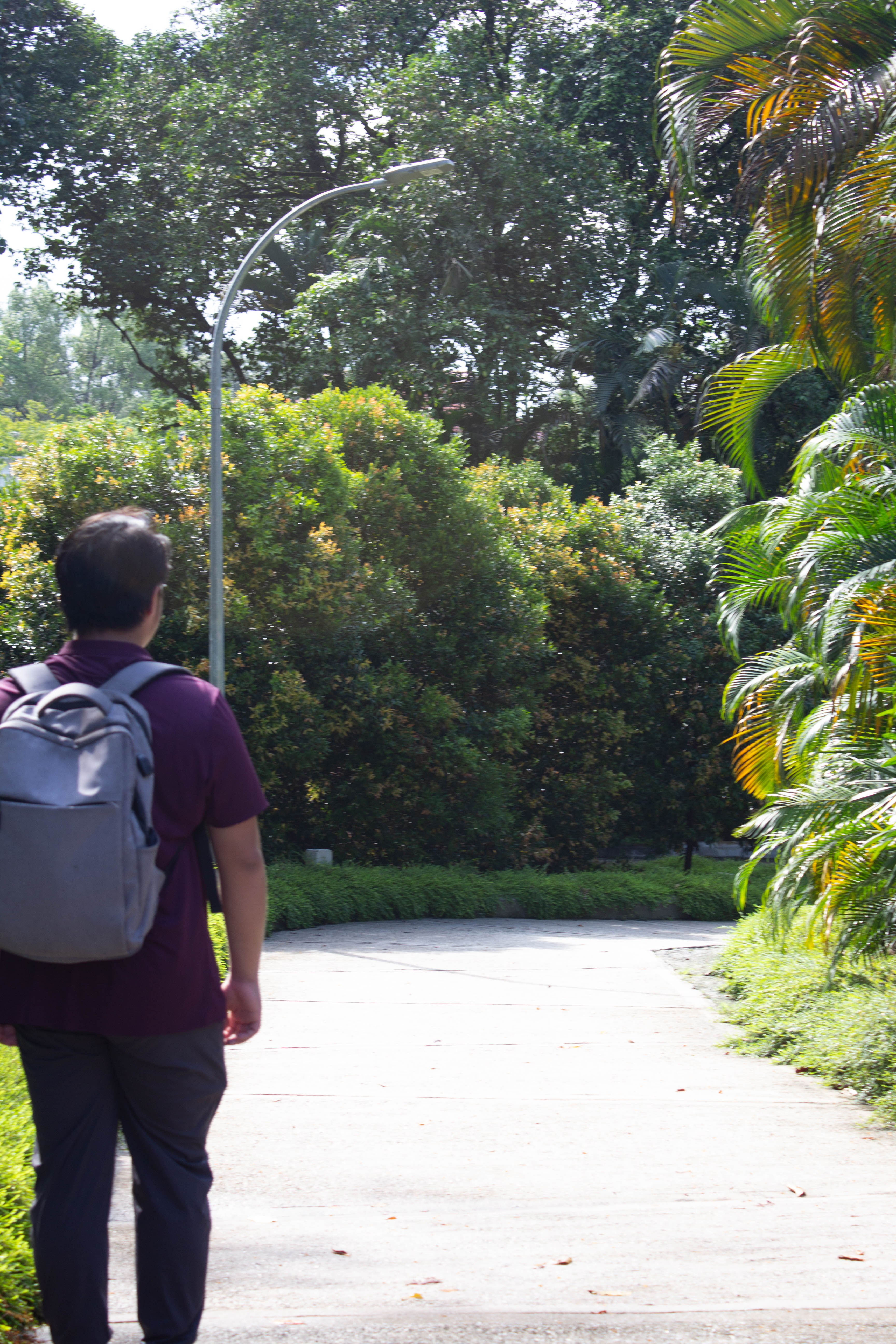
I decided to use this picture because there are tall tapered pillars in my college library with a slight bend which looked similar to the tangent function. In order to model the edge of the pillar, I recognized that it was quite close to resembling a tangent function; therefore, the parent function that I would choose is \( y = \tan(x) \).
In considering the direction in which the curve was pointing in the image, I realized that the curve had to be less steep than that of the parent function. Therefore, a combination of vertical compression and horizontal stretch would be required in order to accommodate for the gradual taper of the pillar. In the beginning, it proved difficult to find the right factors due to the fact that the graph was located too far from the origin. In order to get rid of this difficulty, I decided to shift the graph temporarily to align it in such a way that the middle point of the height of the pillar was located at the origin. This way, it was easier to analyze the curve without taking into consideration its translations.
Now that the shape was known, I translated the graph back to its original position. To do this, I first did a horizontal translation to ensure the midpoint of the curve matched the position of the midpoint in the picture and then translated the graph vertically so that the curve went through important points.
Domain and Range
The domain of the function that I created is:
The reason I restricted my domain to this range is because I only wanted the part of the pillar that was shown in my picture. In retrospect, I probably should have taken a picture where the whole height of the pillar could be seen. This way, I would be able to model the whole curve and not just what could be seen in the picture.
The domain for the parent function \( y = \tan(x) \) and its range are defined as:
\( D: \{x \in \mathbb{R} \mid x \neq \pi/2 + k\pi, \, k \in \mathbb{Z}\} \)
\( R: \{y \in \mathbb{R}\} \)
The above implies that the function is undefined for particular values and has a possibility of having all real numbers as its output. It has vertical asymptotes for such undefined values of \( x \). In my case, after performing the required transformation, the vertical asymptotes have been shifted to \( x = \pi/2 + 2k\pi \). But owing to the fact that the function's domain was limited to a particular finite value lying between the asymptotes, there would not be any undefined part of the function. Therefore, the discontinuity problem does not apply in my case.
Owing to the fact that my function is continuous for the finite domain, the function can have its range found out using the function's value at either end of the domain. Using \( x = \pi/2 \) and \( x = 3\pi/2 \), the approximate values obtained are 2 and 2, respectively. The maximum value for \( y \) obtained is 2.5.
Hence, the range is approximately stated as:
Sine Function
Transformations
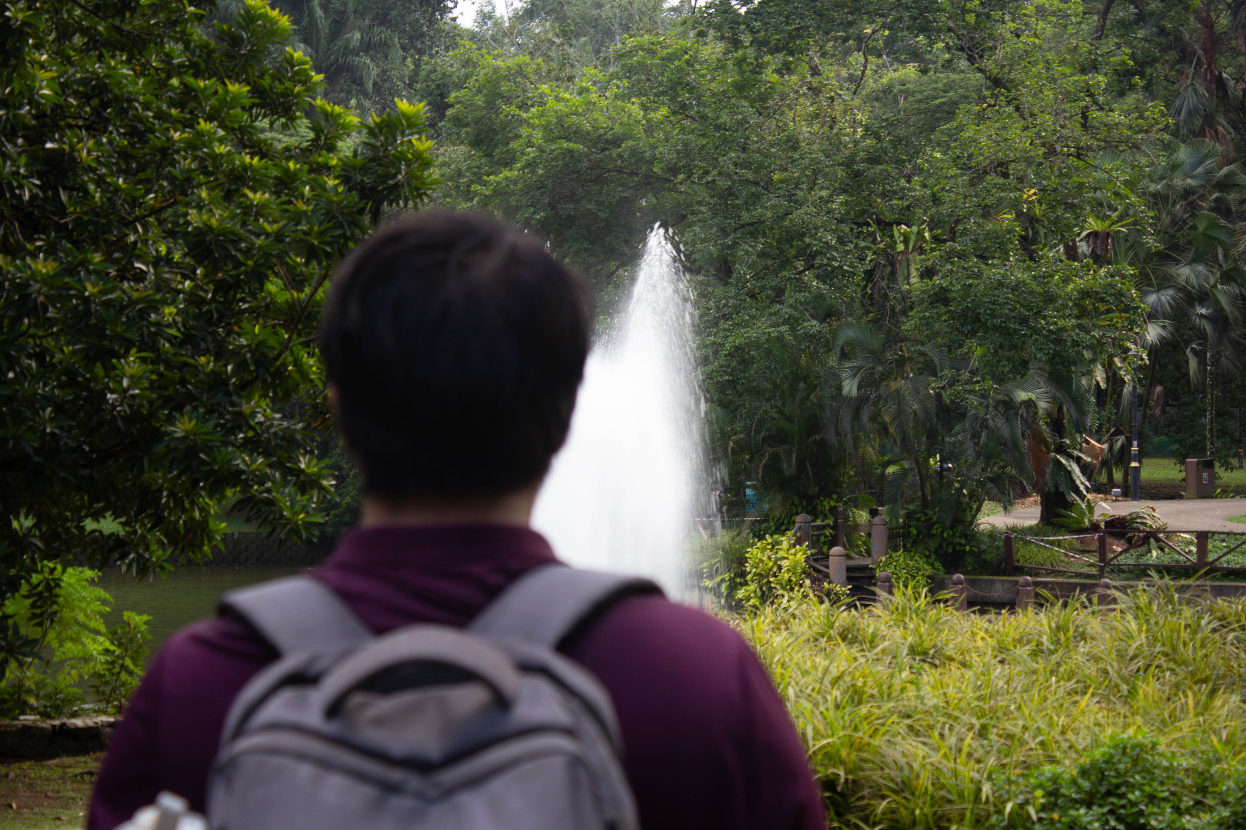
I chose this picture since the waves of the fountain reminded me of a sine wave. In order to describe the shape of this wave using mathematical functions, I first realized that its shape could be represented by a sine function and used \( y = \sin(x) \) as my parent function.
After looking carefully at the shape of the curve in the picture, I realized that it required a horizontal stretch and a vertical stretch in comparison to the parent function. It was initially quite hard for me to find out the right numbers for the stretch due to the fact that the curve on the picture did not start from the origin but was located further away. That is why I temporarily aligned the curve in such a way that the first top was located in the origin and focused only on the shape of the graph. In this way, I figured out that a horizontal stretch and vertical stretch were needed.
After obtaining the correct form of the shape, I moved the graph back to its original form using translations. I translated the graph on the \( x \)-axis such that it had the same coordinates as those in the image and then translated it on the \( y \)-axis so that it went through certain critical points. The resulting function was:
Domain and Range
The domain of the function that I created is:
The domain was set based on the visible portion of the spray in the picture. Looking back, if I had taken a picture where there were two complete waves in the spray, then I could model both of them; but since there is only one half-cycle in the spray visible in the picture, my modeling is based only on what I can see.
The domain of the parent function \( y = \sin(x) \) and its range are defined as:
\( D: \{x \in \mathbb{R}\} \)
\( R: \{y \in \mathbb{R} \mid -1 \le y \le 1\} \)
This implies that the domain consists of all real numbers, whereas the range contains only those from -1 to 1. In addition, the period of the parent function is equal to \( 2\pi \). In this case, after transformations, the period is \( 4\pi \) and the range is \( [-0.5, 2.5] \).
Considering that the function is continuous over the specified interval, we can determine the range using the function values at the endpoints of the domain and at the maximum point of the function. Having calculated the values at \( x = \pi/2 \), \( x = 3\pi/2 \), and \( x = 5\pi/2 \), I received the following outputs approximately equal to 1, 2.5, and 1 correspondingly.
As a result, the range of the function is approximately equal to:
Exponential Decay Function
Transformations
This picture appealed to me because of the exponentially decaying form of the tree branch. In order to represent the edge of the branch, the first step was to note that the form of the branch could be represented by a function of exponential decay and thus, the parent function \( y = 0.5^x \) was chosen.
Based on my observations regarding the orientation of the curve in the image, the curve was decreasing slowly. Therefore, there was a requirement of horizontal stretching to slow down the rate of decay. At first, it was quite hard for me to find the required stretch factor for the horizontal stretch as the graph was located far away from the origin point in the image. So, to make it easier to solve the problem, I made a temporary shift such that the base of the branch would be at the origin point. In this way, I just had to concentrate on the shape and not on translations. After that, based on the rate of change, I concluded that there should be a horizontal stretch and used observation to fine tune the value of stretch.
After establishing the shape, I translated the graph back to its actual position using translations. Specifically, I horizontally translated the graph so that the base of the branch coincided with its actual location and then did vertical translations so that some of the points coincide.
Domain and Range
My function's domain is:
I restricted the domain to the branch length that could be seen from the picture. However, on retrospect, I would have photographed the entire length of the branch, which would allow me to generate a curve that fits the entire branch and not just the visible part of it. This means that my model applies to only the visible part of the branch.
The domain of the parent function \( y = 0.5^x \) and its range are given by:
\( D: \{x \in \mathbb{R}\} \)
\( R: \{y \in \mathbb{R} \mid y > 0\} \)
The function can have any input from the set of real numbers and will yield an output greater than 0 for all such inputs. It will also have a horizontal asymptote at \( y = 0 \). With the transformations, my equation has a horizontal asymptote at \( y = 1 \). But as I have restricted the domain to a small set lying completely above the asymptote, this aspect of the graph is not seen in my case.
The function being continuous on the interval, the range can be found using the outputs generated when substituting values of the endpoints of the domain. When substituting \( x = 1 \) and \( x = 7 \) into the function, I got approximate outputs of 2 and 1.125 respectively.
The range of the function is therefore approximately:
Logarithmic Function
Transformations
I decided to choose this picture due to the fact that the shape of the shade of my desk lamp was similar to the logarithmic graph. The first thing that should be done for modeling the edge of the shade is determining the kind of the graph. As we can see, it corresponds to the logarithmic graph, so the parent function will be \( y = \log(x) \).
Having analyzed the behavior of the graph, I noticed that it is going from right to left. It means that there is a reflection about the \( y \)-axis. Therefore, the new function is \( y = \log(-x) \). At first, it seemed to me to be very hard to find the vertical stretch or compression coefficient since the graph is far from the point of origin and it is not easy to make a comparison in terms of steepness. Thus, I decided to move the image to the point of origin and consider it without translations. After that, having compared the slope of the graph, I realized that it was necessary to compress it vertically.
After determining the shape of the curve, I moved the graph back into its original position using translations. In order to move the graph, I translated it vertically so that it would pass through specific points on the curve. This yielded the following equation for the graph:
This function is very similar to the one shown in the photo of the lamp shade.
Domain and Range
Domain of the function:
I restricted the domain to the part of the lamp shade which could be seen in the picture. If I were to take a new picture, it would have been one that covers the entire lamp shade, which will enable me to construct the entire curve. This means that the current model I have constructed is only applicable for the shaded area in the picture.
The parent function \( y = \log(x) \) has the following domain and range:
This means that the function can accept all positive values and generate any real output. Additionally, it has an undefined point at \( x = 0 \). After applying transformations, my function will have an undefined point at \( x = 2 \). However, I restricted the domain to a very small interval that does not include this undefined value. Hence, I do not have to address this discontinuity in describing the domain and range of the given problem.
Because the function is continuous within the domain, the range can be found through its evaluation at the two extreme values. The result is as follows:
\( x = 1.2 \rightarrow y \approx 2.8 \)
\( x = 1.9 \rightarrow y \approx 2.08 \)
Therefore, the range is approximately as follows:
Absolute Value Function
Transformations
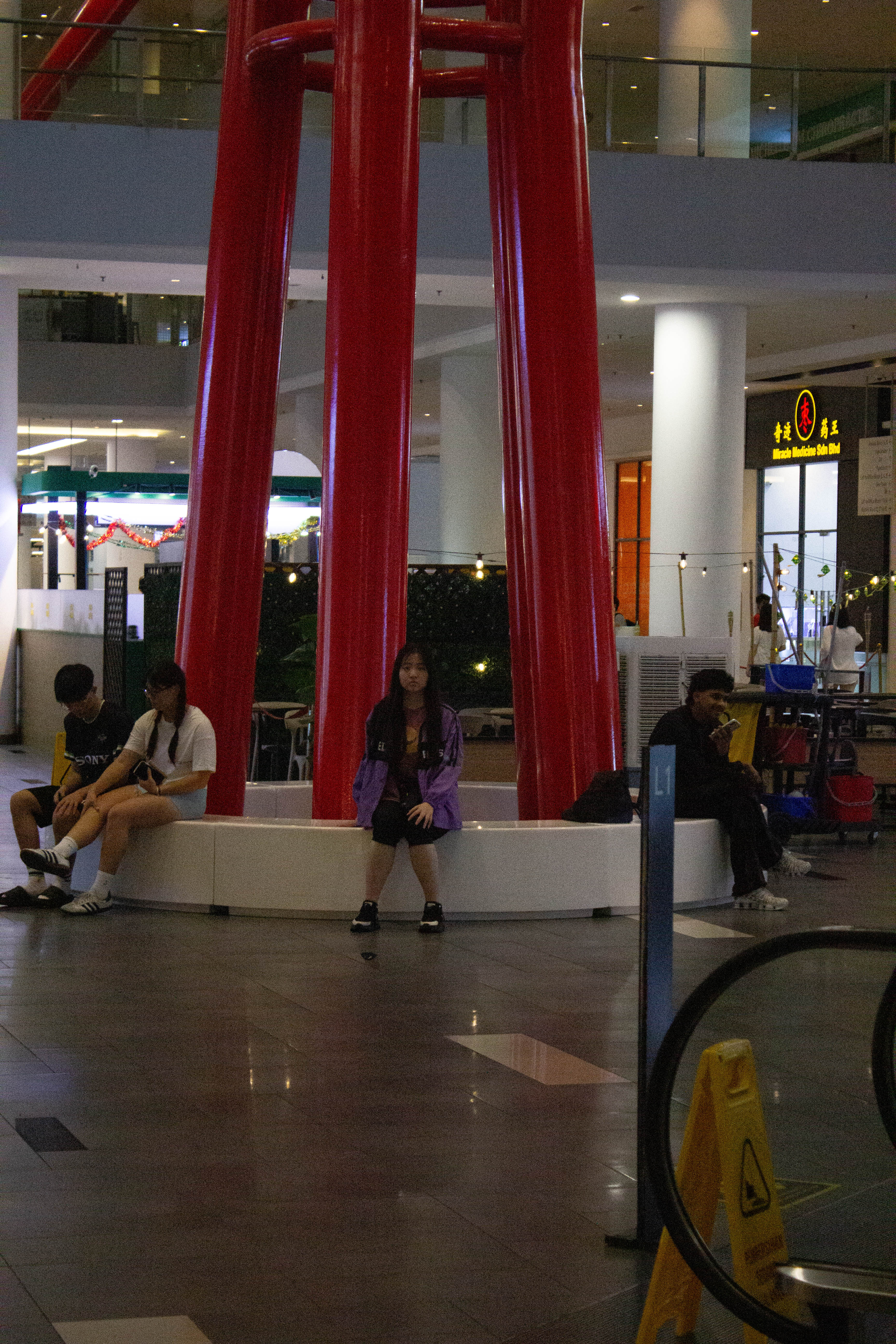
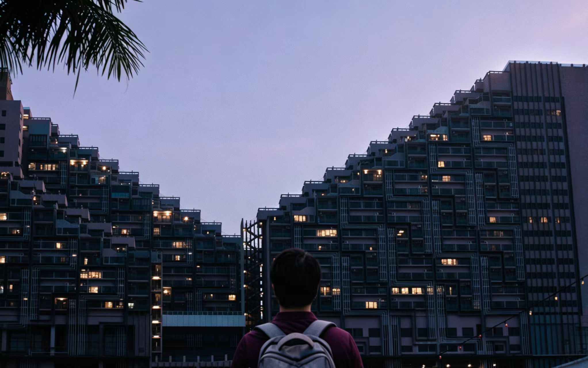
I selected this picture since the clear-cut, symmetrical V-shape of the sign resembled the absolute value graph. The process of determining the shape of the sign required recognizing that it was similar to the parent graph \( y = |x| \). Since the curve in my picture was stretched out horizontally, a stretch would be needed to represent the angle of the sign's opening.
[Note: Text content partially cut off in original manuscript during transformation optimization.]
Domain and Range
The domain of my function is:
I restricted the domain to the part of the sign which I could see in the photograph. With hindsight, I should have positioned the photograph such that it showed the whole V shape, enabling me to graph the entire shape rather than just the visible bit. The reason why I would do so is because, through doing so, my model will reflect the whole V shape.
The domain of the parent function and its range are defined as:
In other words, the parent function produces real values, but the lowest possible value that it can produce is zero. Furthermore, the vertex of the parent function lies at \( (0, 0) \). After the transformation, the vertex of my function lies at \( (3, -1) \). The fact that it is a continuous function over this restricted domain means that to get the range, all I need is to evaluate it over this interval. From evaluating it at \( x = 1 \), \( x = 3 \), and \( x = 5 \), the approximate outputs I get are \( 0 \), \( -1 \), and \( 0 \), respectively.
Quadratic Function
Transformations & Equation
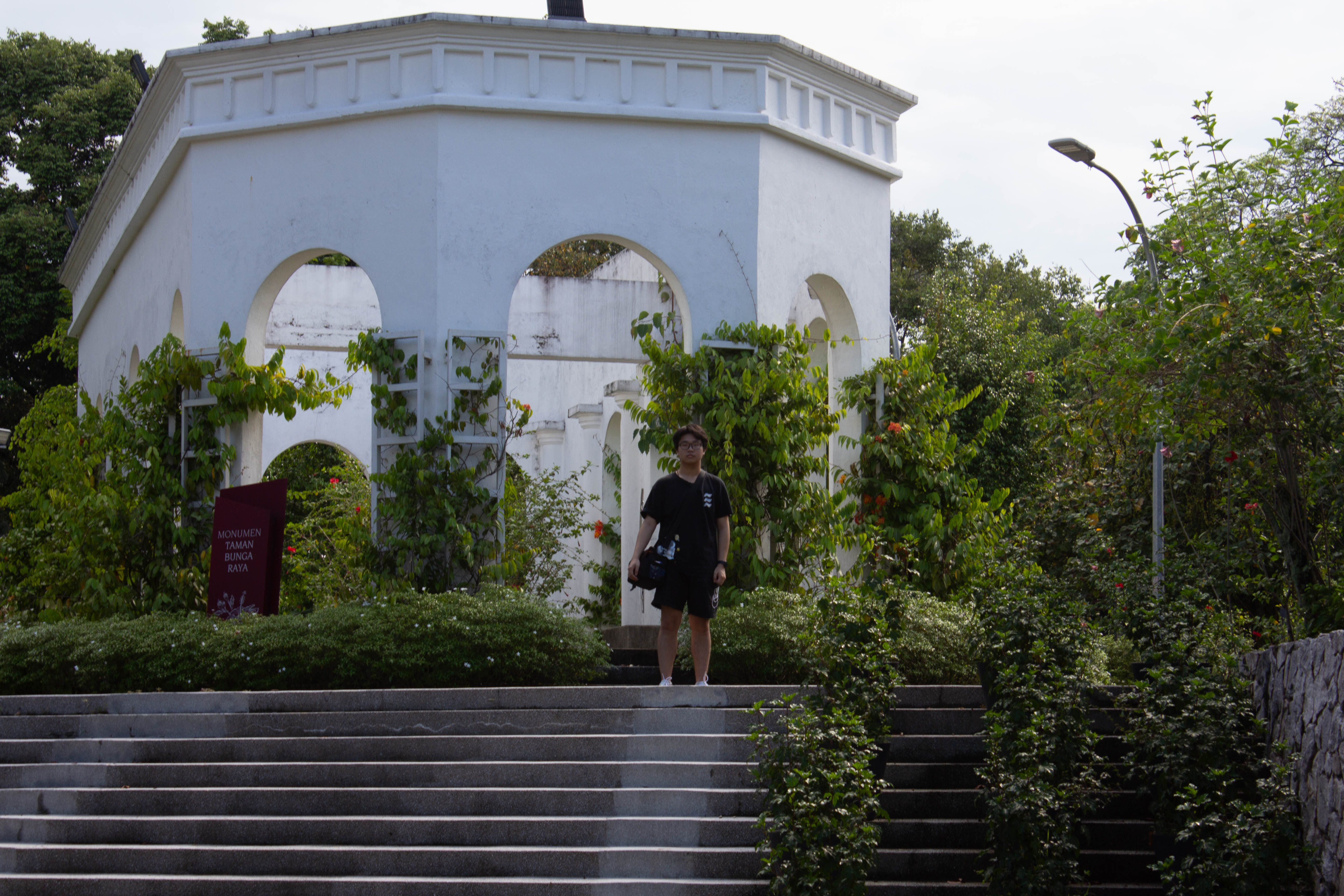
To model the archway, a quadratic function was utilized:
which closely models the shape of the archway in the photograph.
Domain and Range
The domain of my function is:
I restricted the domain of my function to include only the part of the archway that was shown in the picture. Now after completing the assignment, I would make sure to take the picture including the entire arch to get the curve of the whole arch. Hence, the function would be applicable only for the part of the arch that is shown in the picture.
The parent function \( y = x^2 \) has the following domain and range:
The above function is valid for all real values of \( x \) and provides any non-negative real value for output. Its vertex is at point \( (0, 0) \).